Using Ranking Functions to Partition and Order Unfamiliar Data
By Jeffry Schwartz | Expert
How many times have you had to subdivide, group, rank, and organize data when you knew very little about the data itself except for the meanings of the columns? This dilemma is one that the members of the SQLRx team encounter frequently. When a customer requests help with a performance problem, we often do not know the number of databases, tables, or indices (or how busy any of them are) before we begin our analysis of the performance data. We also do not know beforehand which metrics will provide the most insight into a customer’s problems. The unknown nature of the data necessitates that we make no assumptions and therefore, look at all performance data.
To expedite our analyses, we developed Reporting Services routines that enable us dynamically to depict the data graphically. This is particularly useful for processing data from the SQL Server DMVs, which can produce voluminous amounts of data. For example, a simple 12-hour collection can produce millions of data records that are written periodically and efficiently by our T-SQL scripts into flat files for post-processing off-site. To put the analysis problem into better perspective, it is instructive to consider how one might graph the single-record lookups metric for the 6,035 possible database/table/index combinations contained in the Index Operational DMV data used in this article. If every index were used during the data collection period and each graph contained 14 series, this would result in 432 graphs. Obviously, this is unmanageable. Unless some method is devised to place the most interesting series on the first graph or two, the graphs will be as useless as the number columns themselves. A member of our team, Jeff Schwartz, developed some T-SQL code that grouped the data by metric and any other subdivision entity, e.g., instance, database, file, table, or index without resorting to cursors or dynamic SQL. The series were also ranked with the largest N (specified by the user via the Reporting Services UI) maximums on the first graph with the next N series on second graph, etc. The partitioning and ranking mechanism he devised, which employs the DENSE_RANK and ROW_NUMBER T-SQL ranking functions, is applicable to variety of data subdivision and organization problems and is the basis for this article.
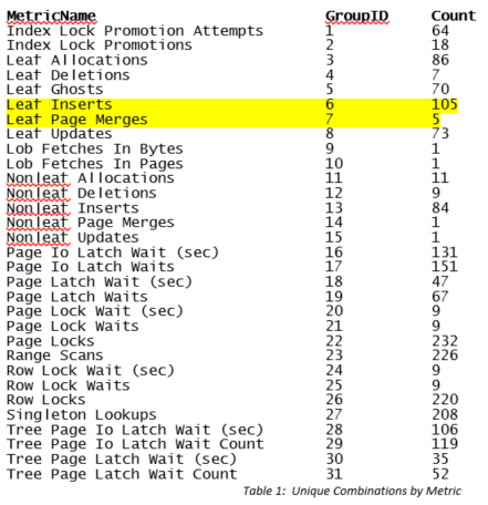
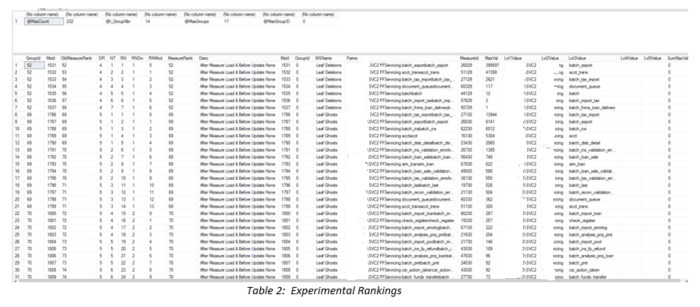
Although the NTILE function appeared to be the obvious choice, Jeff found that he could not obtain the desired metric partitioning for the graphs by using this function. NTILE requires a fixed number of partitions. Some metrics had hundreds of unique series, whereas others had one, seven, or nine (see Table 1). For some combinations, several graphs were created for a given metric, but each graph only had one or two series on it! For those with an intermediate number of combinations, NTILE evenly divided the total number of series into equal portions. This meant that although the user specified a series per graph value such as seven, each graph would only contain five series on it (illustrated in Table 2 by the Leaf Ghosts records), thereby effectively ignoring the user specification. The query below, whose output is shown in Table 1, determines how many unique column combinations existed in the data for each metric. Clearly, the number per metric varied greatly. Please also note that the GroupID was assigned automatically based upon the order by clause within the DENSE_RANK function. This will become an integral part of the final partitioning strategy.
SELECT MetricName, DENSE_RANK() OVER(ORDER BY MetricName) AS GroupID, COUNT(*) AS [Count]
FROM MeasureBeforeUpdate
GROUP BY MetricName
ORDER BY MetricName
The next task was to reestablish the ordering for all the graphs with the worst ones on the first graph, the next worst on the second, etc. After a fair amount of experimenting, Jeff hit upon the following combination that does the entire grouping, ranking, splitting, etc. all in one pass as shown below (it also uses a CTE to simplify the coding and improve legibility). The example below shows all the building blocks so you can see how the final query was derived. For the sake of comparison, ALL attempted ranking variations are shown in the query. The ones that proved useful, DR and RNDiv, are highlighted. along with the combined item named MeasureRank. To aid with interpretation, @I_GroupNbr specifies the number of series per graph provided by the user, @MaxCount determines the largest number of combinations (Count in Table 1), and @MaxGroups specifies the maximum number of possible groups for each metric. This value is computed earlier in the stored procedure to simplify the computations greatly and is established using the following formula: SET @MaxGroups = CEILING (@MaxCount * 1.0 / @I_GroupNbr). The DENSE_RANK function provided the metric groupings, and the ROW_NUMBER function partitioned the columns by metric and ordered them by the maximum value in descending order. The integral division enabled maintaining the relative ranking within a group. The query output is shown below.
WITH RankingList AS (
SELECT MsId,
@MaxGroupID + (DENSE_RANK() OVER (ORDER BY MetricName) – 1) * @MaxGroups +
NTILE(@MaxGroups) OVER (PARTITION BY MetricName ORDER BY MetricName)
AS [OldMeasureRank],
DENSE_RANK() OVER (ORDER BY MetricName) AS DR,
NTILE(@MaxGroups) OVER (PARTITION BY MetricName ORDER BY MetricName) AS NT,
ROW_NUMBER() OVER (PARTITION BY MetricName ORDER BY MaxVal DESC) AS RN,
((ROW_NUMBER() OVER (PARTITION BY MetricName ORDER BY MaxVal DESC) – 1) / @I_GroupNbr) + 1 AS RNDiv,
(ROW_NUMBER() OVER (PARTITION BY by MetricName ORDER BY MaxVal DESC) – 1) % @I_GroupNbr AS RNMod,
@MaxGroupID + (DENSE_RANK() OVER (ORDER BY MetricName) -1) * @MaxGroups + ((ROW_NUMBER() OVER (PARTITION BY MetricName ORDER BY MaxVal desc) -1) / @I_GroupNbr) + 1 AS [MeasureRank]
FROM MeasureBeforeUpdate
)
SELECT GroupId = RankingList.MeasureRank, RankingList.*, MeasureBeforeUpdate.*
FROM MeasureBeforeUpdate
INNER JOIN RankingList ON RankingList.MsId = MeasureBeforeUpdate.Msid
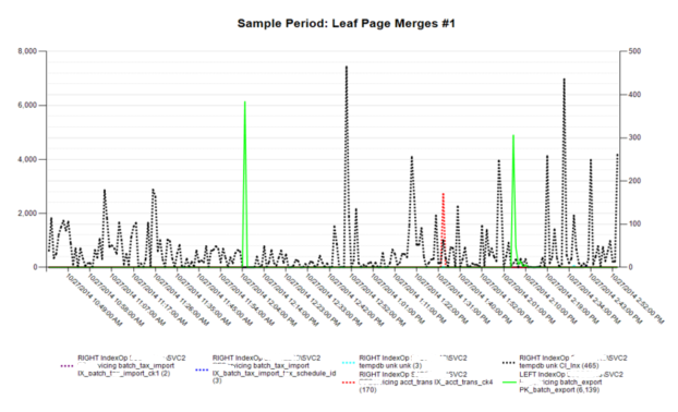
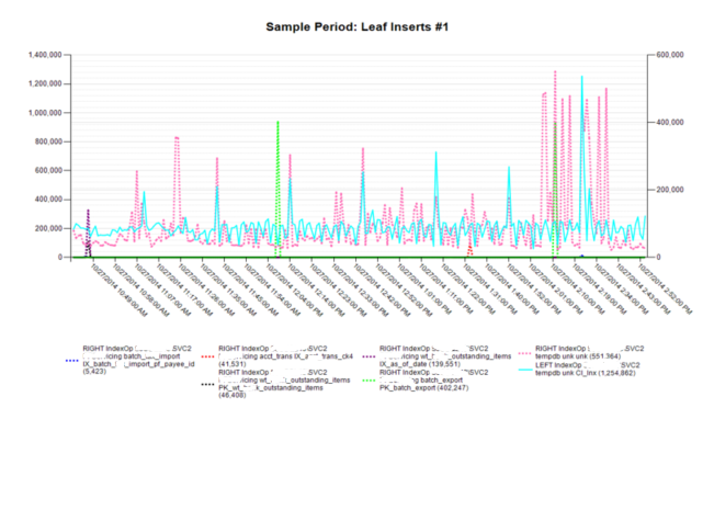
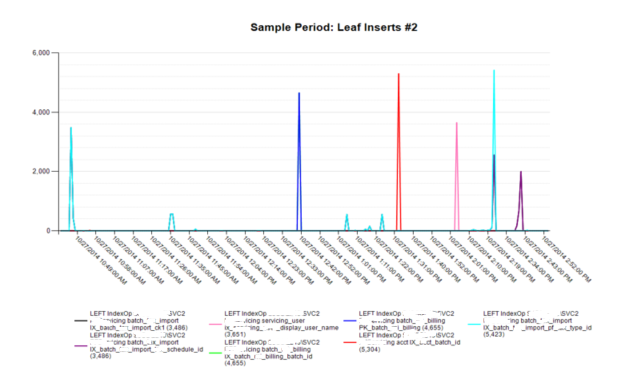
The final code compares the original partitioning code values with those of the new method. The biggest differences involve the replacement of NTILE with ROW_NUMBER and the addition of integral division. This combination automatically numbers the series for a given group and resets this number once it hits the maximum number of items to be shown on a Reporting Services page. Since this is a parameter specified by the user, it now breaks the output up into N sections depending upon how many series are requested for each graph. Examples of the graphs with the number of series per graph specified to be seven are shown below the query. As highlighted in the Table 1, only five Leaf Page Merges combinations existed, whereas there were 105 for Leaf Inserts. As a result, only one graph was needed for the first metric, but 15 were possible for the second. Since each graph set has its own ID (as displayed in the graph titles), it is trivial to terminate the graph generation process early by avoiding the calls for any group greater than a certain value. When returning large numbers of metrics, e.g., 40 for Index Operational statistics, being able to terminate graphing early, e.g., at two, can result in a reduction of more than 93 percent in graph generation duration. With this particular data, the total possible number of graphs was 907, whereas by stopping at only two graphs per metric, the total decreased to 61.
WITH RankingList AS (
SELECT MsId,
@MaxGroupID + (DENSE_RANK() OVER (ORDER BY MetricName) – 1) * @MaxGroups + NTILE(@MaxGroups) OVER (PARTITION BY MetricName ORDER BY MetricName) AS [OldMeasureRank],
@MaxGroupID + (DENSE_RANK() OVER (ORDER BY MetricName) -1) * @MaxGroups + ((ROW_NUMBER() OVER (PARTITION BY MetricName ORDER BY MaxVal DESC) -1) / @I_GroupNbr) + 1 AS [MeasureRank]
FROM MeasureBeforeUpdate
)
SELECT GroupId = RankingList.MeasureRank, RankingList.*, MeasureBeforeUpdate.*
FROM MeasureBeforeUpdate
INNER JOIN RankingList ON RankingList.MsId = MeasureBeforeUpdate.Msid
This article illustrated the pros and cons of using various ranking functions, especially in combination, which is seldom shown in ranking code examples. This article provides a different perspective regarding Windows ranking functions and their use in solving everyday partitioning, ranking, and organization problems.
For more information about blog posts, concepts and definitions, further explanations, or questions you may have…please contact us at SQLRx@sqlrx.com. We will be happy to help! Leave a comment and feel free to track back to us. Visit us at www.sqlrx.com!